Using CCN to train digit recognition

Convolution neural network is known as the most accurate model to train the digit recognition, When in college , we learned laplace transformation in convolution therem . Well I think everyone has return that knowledge to your teacher and leave nothing in your brain. That's ok . So am I. However, we don't need to implement the CNN from stratch and train the data. The keras has already done the model so that we can easily use to trigger the traing in just a few steps.

1. Import Data

import keras
import pandas as pd
from keras import backend as K
from keras.models import Sequential
from keras.layers import Dense, Dropout,Flatten
from keras.layers import Conv2D, MaxPooling2D
from sklearn.model_selection import train_test_split

# Import Data
dataset = pd.read_csv("train.csv")
target = dataset.iloc[:,0].values.ravel()
train = dataset.iloc[:,1:].values
test = pd.read_csv("test.csv").values.reshape(-1,28,28,1)

data_x = train # feartures
data_y = target # targets

x_train, x_test, y_train, y_test = train_test_split(data_x, data_y, test_size=0.2, random_state=42) # split the data
print (x_train.shape);

(33600, 784)

2.Reshape Data

Reshaping data is important as the CNN in Keras only can take data with certain shape. So we have no chices but to reshape the input data.

# 10 numbers 

num_classes = 10  

# input image dimensions
img_rows, img_cols = 28, 28

if K.image_data_format() == 'channels_first':
    x_train = x_train.reshape(x_train.shape[0],1,img_rows,img_cols)
    x_test = x_test.reshape(x_test.shape[0],1,img_rows,img_cols)
    input_shape = (1,img_rows,img_cols)  # 3 = RGB， 1 = black & white
    print (input_shape)
else:
    x_train = x_train.reshape(x_train.shape[0],img_rows,img_cols,1)
    x_test = x_test.reshape(x_test.shape[0],img_rows,img_cols,1)
    input_shape = (img_rows,img_cols,1)
    print (input_shape)


(28, 28, 1)


3. Transfer the integer into 0~1 decimal numbers






# 0~1 float

x_train = x_train.astype("float32")
x_test  = x_test.astype("float32")
x_train /= 255
x_test  /=255 

print('x_train shape:', x_train.shape)
print(x_train.shape[0], 'train samples')
print(x_test.shape[0], 'test samples')





4. Set some basic params for the CNN

y_train = keras.utils.to_categorical(y_train,num_classes) # one-hot encoder
y_test = keras.utils.to_categorical(y_test,num_classes) # one-hot encoder

model =Sequential()
model.add(Conv2D(32, kernel_size=(3,3), activation='relu',input_shape=input_shape)) #32C3
          
model.add(Conv2D(64, kernel_size=(3,3), activation='relu')) #64C3

model.add(MaxPooling2D(pool_size=(2,2))) #MP2
model.add(Dropout(0.25))

model.add(Flatten())
model.add(Dense(128,activation='relu')) # Dense must has Flatten in front ,                                 Total Chain : 6C5-MP2-16C5-MP2-120C1 (FLATTEN) -84N-10N

model.add(Dropout(0.5))
model.add(Dense(num_classes,activation='softmax'))

model.compile(loss=keras.losses.categorical_crossentropy,
              optimizer=keras.optimizers.Adadelta(),
              metrics=['accuracy'])







5. Train the model



The batch_size and epoch are needed to be tuned, here I just randomly give 2 number for demostration.

history = model.fit(x_train, y_train, batch_size=200, epochs=12, verbose=1, validation_data=(x_test, y_test))
score = model.evaluate(x_test, y_test, verbose=0)



6. Draw a graph

%matplotlib inline

import matplotlib
import matplotlib.pyplot as plt


plt.xlabel('x')
plt.ylabel('y')
plt.title('accuracy graph')

plt.plot(range(len(history.history['val_acc'])), history.history['val_acc'])

plt.show()

7.Predict

y_pred = model.predict_classes(test) ## predict, = predict

np.savetxt('CNN_6.csv', np.c_[range(1,len(test)+1),y_pred], delimiter=',', 
           header = 'ImageId,Label', comments = '', fmt='%d')

Well, Why not upload your CNN_6.csv to kaggle to see how the result goes . If the params are properly given , the result should be good enough.

A good table structure can avoid all tunings.

       is the recommendation i give for this topic.

Table structure design is the first step for people to create an application. However becuase some company / people has limited knowledge on database, when their application was put in production, It has bugs and errors here and there. And the oracle is keep releasing from  8i 9i 10G 11G 12C onwards, some bugs has been fixed , some algorithums has been improved, they are still blur on that . 

One obvious case in my work,  when in 10G , the data type char and Varchar2 have some efficiency issues which make these 2 data type different . Thus DBA in oracle 10G are more apt to char rather than varchar2, However, in 11G which is the version i am current using , this problem has been fixed by Oracle , so varchar2 has a better performance than char and also can tolerate a longer String length. And char has been put in the deprecated list in later releases. When I see the table design by our DBA , they are still using char to improve certain performance. Similar cases appear very often . 

In this article , I won't dig so much on these details ,  I will share some important points on table design and how these points can affect queries.

Index Foreign key : 

If tables linked by pri-for key, then don't remember add index on foreign key.

3 ways of Oracle partitioning : 

• range partitioning
• list partitioning
• hash partitioning

3 combined ways of partitioning:

• range-range
• list-list
• list-hash

2 types of index :

• local index , index on partitons : create index .... local;
• global index, index on tables

Why do we need to create partitions?

Because , we can narrow down the scan range when we query so as to improve the speed, Also, It's easier to clean those partitons (truncate, drop, split,add,exchange), Delete will occupy lots of rollback segments writing into undo tablespace those deleted data. so when we clean partitions, we don't need to delete the whole table , so it is very convenient. 

eg:

Alter table t truncate/drop p1; 
Alter table t split partition p_default at 3000 into (partition p3,partition p4);
Alter table t add partition p6 values less than (6000); // delete maxvalue before do it
Alter table t1 exchange partition p1 with table t2 including indexes update global indexes; // exchange data between 2 tables. 

partition table & rowid : when you do an update in partition table, the rowid will be changed as well.
Global tempprary table : auto-cleased when session is closed or transaction is commited
IOT and cluster table : when query an IOT , it won't query from your original table , add index in columns with order by and foreign key.

Primary key : this is just (an index + a constrain), we can directly change an index into a primary key.

Alter table t add  constraint ord_pk primary key(order_id,item_id) using index ord_idx;

Table compression : This will decrease the logic read but increase the CPU.

Alter table t move compress;
Execute dbms.gather_table_stats(ownname=>user,tabname=>'T');
Select table_name, blocks, cp,ression from user_tables where table_name='T';

Never use char and long .

Drop truncate add spilt exchange // this will make index invalidated
Alter table table1 drop partition p1 update global indexes; // this can avoid index invalidated
Alter index idx_par_1 rebuild partition p3; //rebuild local index

collect statistics :

Alter session set statstics_level=all;
Select * from t1,t2 where t1.id=t2.t1_id;
Select * from table(dbms_xplan.display_cursor(null,null,'allstats last'));

Replace delete table with global temporary table:

This can reduce the blow of redo log .

Create global temporary table t_global (id int, col2 int) on commit delete rows;
Insert into t_global.....
//other manipulations ....
commit;

In real situation , we wrote some script to monitor rather than wait for the problems to come out . Scripts are too long to share here, if you have any problem ,please leave a msg.

StratifiedKFold vs Normal KFold

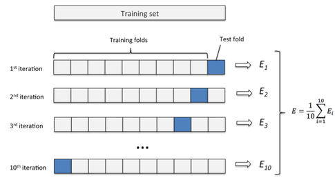
StratifiedKFold is a kind of advanced KFold， the Normal KFold process is as below as we know.

x_data = np.array([[1,2],[2,4],[3,2],[4,4],[5,4],[6,2],[7,4],[8,4],[9,2],[10,4],[11,2],[12,4],[13,2],[14,4],[15,4]
                  ,[16,2],[17,4],[18,4],[19,2],[20,4]])
y_data = np.array([1,2,3,4,5,1,2,3,4,5,1,2,3,4,5,1,2,3,4,5])

kf = KFold(n_splits=10)

for train_index, test_index in kf.split(x_data):
    x_train = x_data[train_index]
    y_train = y_data[train_index]
    x_test = x_data[test_index]
    t_text = y_data[test_index]
    print ("train:{0}  test:{1}".format(train_index,test_index))
    
    # train model
    # test model 
    # get error rate

train:[ 2  3  4  5  6  7  8  9 10 11 12 13 14 15 16 17 18 19]  test:[0 1]
train:[ 0  1  4  5  6  7  8  9 10 11 12 13 14 15 16 17 18 19]  test:[2 3]
train:[ 0  1  2  3  6  7  8  9 10 11 12 13 14 15 16 17 18 19]  test:[4 5]
train:[ 0  1  2  3  4  5  8  9 10 11 12 13 14 15 16 17 18 19]  test:[6 7]
train:[ 0  1  2  3  4  5  6  7 10 11 12 13 14 15 16 17 18 19]  test:[8 9]
train:[ 0  1  2  3  4  5  6  7  8  9 12 13 14 15 16 17 18 19]  test:[10 11]
train:[ 0  1  2  3  4  5  6  7  8  9 10 11 14 15 16 17 18 19]  test:[12 13]
train:[ 0  1  2  3  4  5  6  7  8  9 10 11 12 13 16 17 18 19]  test:[14 15]
train:[ 0  1  2  3  4  5  6  7  8  9 10 11 12 13 14 15 18 19]  test:[16 17]
train:[ 0  1  2  3  4  5  6  7  8  9 10 11 12 13 14 15 16 17]  test:[18 19]

Well , you may notice that the test data don't give a complete categorization . only 2.

However for the stratifiedKFold, it's as below:

x_data = np.array([[1,2],[2,4],[3,2],[4,4],[5,4],[6,2],[7,4],[8,4],[9,2],[10,4],[11,2],[12,4],[13,2],[14,4],[15,4]
                  ,[16,2],[17,4],[18,4],[19,2],[20,4]])
y_data = np.array([1,2,3,4,5,1,2,3,4,5,1,2,3,4,5,1,2,3,4,5])

# in each fold , test set will contain 1,2,3,4,5 completed data, so K is set maximumly to 4 here
kf = StratifiedKFold(n_splits=4)

for train_index, test_index in kf.split(x_data,y_data):
    x_train = x_data[train_index]
    y_train = y_data[train_index]
    x_test = x_data[test_index]
    t_text = y_data[test_index]
    print ("train:{0}  test:{1}".format(train_index,test_index))
    
    # train model
    # test model 
    # get error rate

train:[ 5  6  7  8  9 10 11 12 13 14 15 16 17 18 19]  test:[0 1 2 3 4]
train:[ 0  1  2  3  4 10 11 12 13 14 15 16 17 18 19]  test:[5 6 7 8 9]
train:[ 0  1  2  3  4  5  6  7  8  9 15 16 17 18 19]  test:[10 11 12 13 14]
train:[ 0  1  2  3  4  5  6  7  8  9 10 11 12 13 14]  test:[15 16 17 18 19]

Now, It's very comprehensive. So normally we choose StratifiedKFold rather than Normal KFold.

Add K-Fold Validation to neural network

Last article , I have descussed how to use sequential neural network to train the digit recognition , but re we didn't add cross validation in , so the result may varies . Here I will describe some params to better tune your model . by the way, I will add more hidden layers this time . This is also a way to improve your socre

import keras
from keras.models import Sequential
from keras.layers.core import Dense, Dropout, Activation

Define the model : 

model  = Sequential() # adopt sequential neural model

#input layer
model.add(Dense(64, input_shape=(64,))) # Dense with 64 features
model.add(Activation("relu"))

#hidden layer 1 
model.add(Dense(160))
model.add(Activation("relu"))

#hidden layer 2 
model.add(Dense(160)) 
model.add(Activation("relu"))

#hidden layer 3
model.add(Dense(160))
model.add(Activation("relu"))

#hidden layer 4
model.add(Dense(160))
model.add(Activation("relu"))

# output layer
model.add(Dense(10)) # 10 categories
model.add(Activation("softmax")) # only can output 1 & 0

model.compile(optimizer='adam', loss='categorical_crossentropy', metrics=["accuracy"])

Read data & train :

from sklearn.datasets import load_digits
from keras.utils import np_utils

digit = load_digits() # here we use another embeded dataset called digits 

data_x = digit.data
data_y = np_utils.to_categorical(digit.target, 10) # convert to one-hot-encoder

train_x = data_x
train_y = data_y

# k-fold crossvalidation is added with a split point at 20% 80%
history = model.fit(train_x, train_y, epochs=200,  verbose=1, validation_split= 0.2) 

print (history.history['acc'])
print (history.history['loss'])

Here we all one parameter called validation_split, it will split the dataset into 80% training set and 20% test set to do the corss validation , It is not using the normal k-fold , it is using one called StratifiedKFold so that the accurancy will be more accurate.

Visualise to Tune :

%matplotlib inline

import matplotlib
import matplotlib.pyplot as plt


plt.xlabel('x')
plt.ylabel('y')
plt.title('acc graph')

plt.plot(range(len(history.history['val_acc'])), history.history['val_acc'])

plt.show()

This graph shown is the corss- validation graph which will be more precise .

In the end , you may think whether there exist a way to persist the model which i can use next time . What I can tell you is Yes.

Persist the model :

import h5py
from keras.models import load_model

model.save('model.h5') # persist the model to external file

model2 = load_model('model.h5') # load the persistent model from external file

Compare the  result  from loaded model with the previous :

y_pred2 = model2.predict(train_x)

y_pred1 = model.predict(train_x)

y_pred1 == y_pred2 # compare the difference, no different

Revert data from one-hot-vector back :

import numpy as np

# revert one-hot-encoder back to the original formatnp.argmax(y_pred1[1500], axis=0)  # revert one-hot-encoder back to normal digit

1

If anything is unclear for you, please leave a msg.

How to intervene the explain plan !

Sometimes , the explain plan of Oracle is not accurate ,  the way we change the explain plan is called hint, if you randomly write something inside /*asas*/ , well this is just a annotation . Hint will not work at all . if the table has a alias, you must use the alias to hint eg :  (index(t))

Select * from v$sql_hint; // check all the hints

/* + leading(t2) */       // visit t2 firstly
/* + use_nl(t1) */        // t1 is visited lastly after jpin
/* + index(id,object_id) */    // run index, but the index can't be null

Insert all into table1 into table2 select * from t // insert into multiple tables

// write pagination in this way

select * from (select t.*, rownum as rn from t t where rownum <=10) a where a.rn >= 1 

Update t set object_name = 'abc' where object_id = 8 and t.rowid='agsjgdgsgdhs'// with rowid, it will be very fast

Select /* + result_cache */ count(*) from t //cache results will increase the efficiency very much, it directly read from share pool，if query twice or triple times , logic read is 0

Create materialized view mv_count build immediate refresh on commit enable query rewrite as select count(*) from t; // create materilised view , the speed is faster

select count(*) from t; // this is super fast

Oracle Archiving & Logging

Archive or logging is a great tool to restore a broken database or do desaster recovery in oracle . if you are doing software enginneering , this part is optional.  Now I will give a brief introduction for it.

Redo log  : The redo log in oracle will record down all manipulations so as to do a data recovery in future.

Archive log : when one log file is full, the log accumulation will switch to another log file , log1.arc, log2.noarc ... , then the log files which are full eg: log.arc etc will be archived by a process called ARCH, so in future we can do a desaster recovery following it, this is called archived mode.

In non-archived mode, you can avoid your DB instances dead, but can't avoid hardward broken. Archiving will happen in log switching , of course , manual log switch can also trigger archiving.

Online log : 2or more log files iternate to do hot backup.

If your requirement is to restore your database back to the time : 10 july 12p.m , you can use the archive mode to achieve.

Archive file:

Archive log list // check DB archive mode

how to open archive mode : 
1 startup mount ;
2 alter database archivelog; (alter database noarchivelog // close archive mode)
3 alter database open;

Show parameter db_reco // show archive log saving path
Alter system switch logfile // manual switch log file to trigger archiving

Select * from v$archive_dest; // check archive log's path and status
Select * from v$archive_log // check history archive log

how to change archive directory/path?
Show parameter log_archive_dest; //check your manual setted archiving location
Alter system set log_archive_dest_1 = 'location=D:\songlei\'; // change the archive path
Alter system set log_archive_dest_2 = 'location=D:\songlei2\'// appoint 2 paths to store archive log, so save log into 2 places = hot spare

Alter system set log_archive_dest_state_1 = 'defer'; // defer means this path can't be used

Online log : 2 or more log files in a group , if one is broken , as long as there exist at least one can be read, then this log group can be used.

Select * from v$log;  // check the log group

STATUS :

• current : the oracle is currently using this log group
• active : dirty data in memory hasn't finished writing data into log file
• inactive : dirty data in memory has finished writing data into log file
• unused : it's hasn't been used

Select * from v$logfile // read the specific log file
Alter database add logfile member 'D:\app\Administrator\oradata\orcl\redo02.log' to group 2; 
// add log file into log group，add redo02.log into group 2
Alter database add logfile group 4 'D:\app\Administrator\oradata\orcl\redoGroup04.log' size 10M; // add one log group named redoGroup04.log size is 10M

Alter database clear logfile group [group Number] // erase the whole log file，status must be inactive

All right's that's all about redo log and archive, well it's not so vivid as this command only will be used if you are doing a data recovery in lab. but if you're interested you can still watch some Youtube .

Hope my explaination is ok , if anything is not clear , please leave msg.

Using Comparator to sort

This article will teach you how to use comparator to order your collections, if you don't know this before , It will greatly helps you.

For example , we have an object called paymentVO with lots of fields inside, our requirement is to do ascending or descending order following a field called "paymentSequenceNo"  to show it .

public static void ascendingSort(List<PaymentVO> list) {
 if (!list.isEmpty()) {
     Collections.sort(list,new Comparator() {

     @Override
     public int compare(Object o1, Object o2) {
          PaymentVO nVo1 = (PaymentVO) o1;
          PaymentVO nVo2 = (PaymentVO) o2;
          return nVo1.getBankTradePaymentSeqNo().compareTo(nVo2.getBankTradePaymentSeqNo());

  }});
 }
}

Similarly ,In descending order , Just change Collections.sort(..) to Collections.reverse(...) will do :

public static void desscendingSort(List<PaymentVO> list) {
   if (!list.isEmpty()) {

        Collections.reverse(list,new Comparator() {
        @Override
        public int compare(Object o1, Object o2) {
           PaymentVO nVo1 = (PaymentVO) o1;
           PaymentVO nVo2 = (PaymentVO) o2;
           return nVo1.getBankTradePaymentSeqNo().compareTo(nVo2.getBankTradePaymentSeqNo());

  }});
 }
}

Tuning Table join in Oracle

      is the recomnendation i give. 

Join tables to query in oracle is the most common manipulation that people do in their daily work. However, most of those slow queries or slow applications are due to the some bad joined tables . As software engineer, most of them don't know how to check how their query goes . It's ok. I have learned some when i studied and worked before.

I have summarise some notes to share with you how to tune your query in your work.

Oracle Join types :

• Nested loops join
• Hash Join
• Merge Sort Join

Nested loop join : loop to find and match one by one . It's used in small range scan in OLTP app.

Merge sort/Hash Join : Combine 2 tables to find and match , throw aways the leftover. It is used in massive range scan in OLTP application.

Check number of visit :  set statistic-level = all 

Under nested loop join : 

Starts : how many times this table is visited , very important param

Under Hash join/Merge sort join : The number of visit is alwayse 0 or 1. 

Table sequence and efficiency

When you notice, small table size in nexted loop join should be put before, the bigger table size one should be  put behind.  So  you use small table to find the big table , the number of visit will be less. 

But for Hash Join and Merge join, this doesn't make a difference. 

Table join is ordered ?

Nested loop join and hash join will not sort / order the result (0 sort), Merge sort will do sorting twice and merge in the end. 

Join Limitation ?

Nested loop has no limitation , For Hash join, you can't use < or > or like , only can use = , For Merge sort join, you can't use != , or like . but you can use others like < or >. 

Others :

Nested loop join : create an index in the constraint column where n = 2 ( create index here) , create an index in the constraint of connected table , where t1.id = t2.id ( create an index)

Hash Join : create indexes in all linking constraints in both tables.

Merge sort join : the same as hash join. if the table is visited tons of times , please consider to choose hash join as this will reduce the cost or sortting . 

 

Digit Recognition - Sequential Neural Network in Keras

Last article I have demostrated a basic neural network in digit recognition achieving a 94% accurancy without tuning. Well , this result is not nice. Err.. let's try another neural network to try whether we can increase the accurancy a bit without tuning too much.

Before you run code script , you gotta install the Tensorflow and Keras , those 2 packages. Tensorflow is a neural network-based encapsulation in python , then Keras is a higher encapsulation based on Tensorflow using python. So normally , you of course use the advanced Keras rather than the basic Tensorflow.

import keras
import numpy as np
import pandas as pd
from sklearn import datasets
from keras.models import Sequential
from keras.layers.core import Dense, Dropout, Activation

1. create a model

model  = Sequential() #create a model called sequential

#input layer
model.add(Dense(128, input_shape=(784,)))# Dense is called fully-connected layer with 128 neurons inside
model.add(Activation("sigmoid")) # activation function

#hidden layer
model.add(Dense(160))# Dense is fully-connected layer with 160 neurons inside
model.add(Activation("sigmoid")) #activation function

#output layer
model.add(Dense(10))# Dense is fully-connected layer with 10 neurons
model.add(Activation("softmax")) # output only consist of 0 and 1

model.compile(optimizer='adam', loss='categorical_crossentropy', metrics=["accuracy"])

Hidden layer's neurons' number is a tuning param, so normally , you need to try & error various to see how is the result goes.

Output layer's neuron's number is a fixed number, it depends on your output, eg : digits has 10 numbers from 0 to 9 , so i put 10 there.

2. read & train the data

from keras.utils import np_utils

dataset = pd.read_csv("train.csv")
target = dataset.iloc[:,0].values.ravel()
train = dataset.iloc[:,1:].values
test = pd.read_csv("test.csv").values

train_x = train
train_y = np_utils.to_categorical(target, 10) # convert into one-hot-encoder

# "verbose" is to print the result,  "epoch" is training frequency
history = model.fit(train_x, train_y, epochs=650,  verbose=1) 


print (history.history['acc'])
print (history.history['loss'])

Epoch 1/650
42000/42000 [==============================] - 11s - loss: 0.5749 - acc: 0.8446    
Epoch 2/650
42000/42000 [==============================] - 11s - loss: 0.3669 - acc: 0.8891    
Epoch 3/650
42000/42000 [==============================] - 12s - loss: 0.3301 - acc:

epochs is how many times you want to train your model, this is the param you gotta tune. noramlly just try & error a big number to see whether the graph in the next phase is convergent .if it is converging well, then it proves that this 650 in epochs is a good param.

np_utils.to_categorical is you convert the 0 to 9 , 10 numbers into binary expression , because binary is consiste with only 0 and 1, so it can fill the sigmoid function to feed the model , this is very important.

3.draw a graph to tune the model

%matplotlib inline

import matplotlib
import matplotlib.pyplot as plt


plt.xlabel('x')
plt.ylabel('y')
plt.title('acc graph')

plt.plot(range(len(history.history['acc'])), history.history['acc'])

plt.show()

This Step is the most important , because you only tune your params based on this graph , as you can see, the line is convergent and less fluctuated which means your model's prediction go stable in the later phase . This is a good sign. 

The way you tune your model is to let the graph go as less fluctuated as so possible . So in the end , it go alomost a horizontal line which should be the best result you want to achieve in theory. 

4. draw a sequence diagram and show here

from IPython.display import SVG
from keras.utils.vis_utils import model_to_dot

SVG(model_to_dot(model).create(prog='dot', format='svg'))

This part is to draw a flow chart basicly to see how your model goes, it is not a must. however, it 's good to have.

5. predict

y_pred = model.predict_classes(test) ## predict, = predict

np.savetxt('neural_5.csv', np.c_[range(1,len(test)+1),y_pred], delimiter=',', 
           header = 'ImageId,Label', comments = '', fmt='%d')

27296/28000 [============================>.] - ETA: 0s

Ok the flow is simple and of fun, can't wait to see how the result go , isn't it?

upload the result to kaggle to see how much the result is improved.

It should go between 96 % to 99% depends how do you choose your hidden layer's neurons and epoch's. Anyway, if you find any part is blur for you, please leave a msg

References ：

http://www.graphviz.org/Download_windows.php
https://keras.io/models/sequential/
https://keras.io/layers/core/
https://transcranial.github.io/keras-js/#/