Credit Card Recognition

Credit Card recognition will be based on the modal from OpenCV,  It's not necessary to train our own modal based on data as the card number format are mostly all the same.

1.  download the OpenCV jar file and add into classpath or import as maven, then static import the OpenCV c++ library as below:

static {
        System.loadLibrary(Core.NATIVE_LIBRARY_NAME);
    }

2. read the credit card image into the program into the Mat object

public static void main(String[] args) {
        Mat srcImage = loadImage("img/card.jpg");
}

public static  Mat loadImage(String path) {
 Mat newImage = Imgcodecs.imread(path);
 return newImage;
}

3. turn the card image into grey color (grey scale process)

public static void main(String[] args) {
 Mat srcImage = loadImage("img/card.jpg");
 Mat grey = grey(srcImage);
}

public static Mat grey(Mat srcMat) {
 Mat dest = new Mat (); 
 Imgproc.cvtColor(srcMat, dest, Imgproc.COLOR_RGB2GRAY);
 return dest;
}

4. turn the grey scale image into a black & white image. (binary process)

public static void main(String[] args) 
{
 Mat srcImage = loadImage("img/card.jpg");
 Mat grey = grey(srcImage);
 Mat binary = blackWhite(grey);
}

public static Mat blackWhite(Mat grayMat) {
  Mat binaryMat = new Mat(grayMat.height(),grayMat.width(),CvType.CV_8UC1);
         Imgproc.threshold(grayMat, binaryMat, 30, 200, Imgproc.THRESH_BINARY);
         return binaryMat;
}

5. Erode the black & white image to make the word bolder and clearer so as to be easy to be recognized.

public static void main(String[] args) {
 Mat srcImage = loadImage("img/card.jpg"); 
 Mat grey = grey(srcImage);
        Mat binary = blackWhite(grey);
 Mat erode = imageErode(binary);
}
public static Mat imageErode(Mat srcMat) {
 Mat destMat = new Mat();
 Mat element = Imgproc.getStructuringElement(Imgproc.MORPH_RECT, new Size(3, 3));
        Imgproc.erode(srcMat,destMat,element);
        return destMat;
}

6. crop the key region to remove the noise.

public static void main(String[] args) {
 Mat srcImage = loadImage("img/card.jpg");
 Mat grey = grey(srcImage);
        Mat binary = blackWhite(grey);
 Mat erode = imageErode(binary);
        Mat adjust = filterAndcut(erode);
}
public static Mat  filterAndcut(Mat destMat) {
  int a =0, b=0, state = 0;
         for (int y = 0; y < destMat.height(); y++) //row
         {
             int count = 0;
             for (int x = 0; x < destMat.width(); x++) //column
             {
                 // get the row pixel value 
                 byte[] data = new byte[1];
                 destMat.get(y, x, data);
                 if (data[0] == 0)
                     count = count + 1;
             }
             if (state == 0)//not a valid row
             {
                 if (count >= 150)//find a valid row
                 {//valid row qualify a 10 pixel noise
                     a = y;
                     state = 1;
                 }
             }
             else if (state == 1)
             {
                 if (count <= 150)// find a valid row
                 {//valid row qualify a 10 pixel noise
                     b = y;
                     state = 2;
                 }
             }
         }
         System.out.println("filter upper bound "+Integer.toString(a));
         System.out.println("filter lower bound "+Integer.toString(b));


         //crop the valid region
         Rect rect = new Rect(0,a,destMat.width(),b - a);
         Mat resMat = new Mat(destMat,rect);
         return resMat;
 }

7. recognize and print the result.

public static void main(String[] args) {
  Mat srcImage = loadImage("img/card.jpg");
  Mat grey = grey(srcImage); 
  Mat binary = blackWhite(grey);
  Mat erode = imageErode(binary);
  Mat adjust = filterAndcut(erode);
  
  printResult(matToBufferImage(adjust)); 
}

public static BufferedImage matToBufferImage(Mat grayMat) {
 if (grayMat == null) {
      return null;
 }
 byte[] data1 = new byte[grayMat.rows() * grayMat.cols() * (int)(grayMat.elemSize())];
 grayMat.get(0, 0, data1);
 BufferedImage image1 = new BufferedImage(grayMat.cols(), grayMat.rows(),BufferedImage.TYPE_BYTE_GRAY);                           
 image1.getRaster().setDataElements(0, 0, grayMat.cols(), grayMat.rows(), data1);
 return image1;
}

public static void printResult(BufferedImage src) {
 ITesseract instance = new Tesseract();
 instance.setDatapath("F:/Tess4J-3.4.8-src/Tess4J/tessdata"); // Credit card trained data
 long startTime = System.currentTimeMillis();
 String ocrResult;
 try {
       ocrResult = instance.doOCR(src);
       System.out.println("OCR Result: \n" + ocrResult + "\n spend：" + (System.currentTimeMillis() - startTime) + "ms");
 } catch (TesseractException e) {
       e.printStackTrace();
 } 
}

That's all for this project.

Introductory python code of bayes

This article is a introduction of how to use bayes in python. naive bayes is a probability model/formula which is used under lots of constraints . In reality , I seldom use it as normally data from industrial environment can't fit the bayes' constraints which is "Law of large numbers" and max-lilkelihood normally is build under lots of assumptions which make the model inaccurate.  In this article ,I won't derive the formula as typing math formulas in computer is a terrible work for me. :)

I will use the digit recognition data set from kaggle to demostrate how the basic flow works .

Import libs & datas 

%%time

import numpy as np
import pandas as pd
from sklearn.lda import LDA
from sklearn import datasets 
from sklearn import metrics
from sklearn.model_selection import KFold
from sklearn.naive_bayes import GaussianNB  # import into bayes lib
dataset = pd.read_csv("train.csv")
target = dataset[[0]].values.ravel()
train = dataset.iloc[:,1:].values
test = pd.read_csv("test.csv").values

x_finaltest = test  # test data

kf = KFold(n_splits = 10)

Train & predict in 10 Fold CrossValidation 

total_score1 = []
gnb = GaussianNB()
for train_index ,test_index in kf.split(train):
    x_train = train[train_index]
    y_train = target[train_index]
    x_test  = train[test_index]
    y_test  = target[test_index]
        
    gnb.fit(x_train, y_train)  # train the model
     
    y_predict1 = gnb.predict(x_test)  # predict 

    total_score1.append(metrics.accuracy_score(y_predict1,y_test)) # compare and score

# print average score
print(np.mean(total_score1))

y_pred1 = gnb.predict(x_finaltest) # predict

# save into file
np.savetxt('bayes.csv', np.c_[range(1,len(x_finaltest)+1),y_pred1], delimiter=',', 
           header = 'ImageId,Label', comments = '', fmt='%d')

0.556166666667
Wall time: 4min 32s

Data Visulization

Data visualization is one of the important processes for data analysis. Because sometimes you may need to see whether your tuning goes to the right direction rather than wrong directions which the result looks more blur and abstract. Also, Visulization can help you demostrate your work to client and show your effort to your boss, as we human are visual animals.

Personally , I did seldom visulizations as i think they are too exaggerating and abstract which give few help to my work. But I will still show something in this article .

I will take the example from last article "cnn to train digit recognition" to visulise the convolution kernel and some output there. so the codes below can be appended after the last block following that article.

1. Kernel shape

# visualize weights
import numpy as np
W = model.layers[0].kernel.get_value(borrow=True)
W = np.squeeze(W)
print ("W shape : " , W.shape)

W shape :  (3, 3, 32)

W[:,:,0] # print the content of 1st convolution kernel

array([[ 0.04594247,  0.03799061, -0.1205595 ],
       [ 0.11602765, -0.08880974,  0.04387789],
       [-0.06434739,  0.0857822 ,  0.09397142]], dtype=float32)

2. Visualize the convolution kernel

# draw out the convolution kernel
%matplotlib inline
import matplotlib.pyplot as plt

for i in range(32):
    sub = plt.subplot(4,8,i+1) # row 4, column 8, ith image 
    plt.axis('off')
    sub.imshow(W[:,:,i], cmap=plt.cm.gray)

3. Print the shape after image is convolved by kernel

# output after convolution
import theano

convout1_f = theano.function(model.inputs,[convout1.output])
C1 = convout1_f([x_train[0]])
C1 = np.squeeze(C1)
print("C1 Shape : ", C1.shape)

C1 Shape :  (6, 6, 32)

Here you may need to install the theano by the way.

4. Visualize image after convolved by the kernel

%matplotlib inline
import matplotlib.pyplot as plt

for i in range(32):
    sub = plt.subplot(4,8,i+1)
    plt.axis('off')
    sub.imshow(C1[:,:,i], cmap=plt.cm.gray)

Using CCN to train digit recognition

Convolution neural network is known as the most accurate model to train the digit recognition, When in college , we learned laplace transformation in convolution therem . Well I think everyone has return that knowledge to your teacher and leave nothing in your brain. That's ok . So am I. However, we don't need to implement the CNN from stratch and train the data. The keras has already done the model so that we can easily use to trigger the traing in just a few steps.

1. Import Data

import keras
import pandas as pd
from keras import backend as K
from keras.models import Sequential
from keras.layers import Dense, Dropout,Flatten
from keras.layers import Conv2D, MaxPooling2D
from sklearn.model_selection import train_test_split

# Import Data
dataset = pd.read_csv("train.csv")
target = dataset.iloc[:,0].values.ravel()
train = dataset.iloc[:,1:].values
test = pd.read_csv("test.csv").values.reshape(-1,28,28,1)

data_x = train # feartures
data_y = target # targets

x_train, x_test, y_train, y_test = train_test_split(data_x, data_y, test_size=0.2, random_state=42) # split the data
print (x_train.shape);

(33600, 784)

2.Reshape Data

Reshaping data is important as the CNN in Keras only can take data with certain shape. So we have no chices but to reshape the input data.

# 10 numbers 

num_classes = 10  

# input image dimensions
img_rows, img_cols = 28, 28

if K.image_data_format() == 'channels_first':
    x_train = x_train.reshape(x_train.shape[0],1,img_rows,img_cols)
    x_test = x_test.reshape(x_test.shape[0],1,img_rows,img_cols)
    input_shape = (1,img_rows,img_cols)  # 3 = RGB， 1 = black & white
    print (input_shape)
else:
    x_train = x_train.reshape(x_train.shape[0],img_rows,img_cols,1)
    x_test = x_test.reshape(x_test.shape[0],img_rows,img_cols,1)
    input_shape = (img_rows,img_cols,1)
    print (input_shape)


(28, 28, 1)


3. Transfer the integer into 0~1 decimal numbers






# 0~1 float

x_train = x_train.astype("float32")
x_test  = x_test.astype("float32")
x_train /= 255
x_test  /=255 

print('x_train shape:', x_train.shape)
print(x_train.shape[0], 'train samples')
print(x_test.shape[0], 'test samples')





4. Set some basic params for the CNN

y_train = keras.utils.to_categorical(y_train,num_classes) # one-hot encoder
y_test = keras.utils.to_categorical(y_test,num_classes) # one-hot encoder

model =Sequential()
model.add(Conv2D(32, kernel_size=(3,3), activation='relu',input_shape=input_shape)) #32C3
          
model.add(Conv2D(64, kernel_size=(3,3), activation='relu')) #64C3

model.add(MaxPooling2D(pool_size=(2,2))) #MP2
model.add(Dropout(0.25))

model.add(Flatten())
model.add(Dense(128,activation='relu')) # Dense must has Flatten in front ,                                 Total Chain : 6C5-MP2-16C5-MP2-120C1 (FLATTEN) -84N-10N

model.add(Dropout(0.5))
model.add(Dense(num_classes,activation='softmax'))

model.compile(loss=keras.losses.categorical_crossentropy,
              optimizer=keras.optimizers.Adadelta(),
              metrics=['accuracy'])







5. Train the model



The batch_size and epoch are needed to be tuned, here I just randomly give 2 number for demostration.

history = model.fit(x_train, y_train, batch_size=200, epochs=12, verbose=1, validation_data=(x_test, y_test))
score = model.evaluate(x_test, y_test, verbose=0)



6. Draw a graph

%matplotlib inline

import matplotlib
import matplotlib.pyplot as plt


plt.xlabel('x')
plt.ylabel('y')
plt.title('accuracy graph')

plt.plot(range(len(history.history['val_acc'])), history.history['val_acc'])

plt.show()

7.Predict

y_pred = model.predict_classes(test) ## predict, = predict

np.savetxt('CNN_6.csv', np.c_[range(1,len(test)+1),y_pred], delimiter=',', 
           header = 'ImageId,Label', comments = '', fmt='%d')

Well, Why not upload your CNN_6.csv to kaggle to see how the result goes . If the params are properly given , the result should be good enough.

StratifiedKFold vs Normal KFold

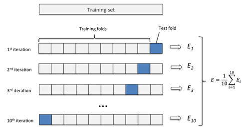
StratifiedKFold is a kind of advanced KFold， the Normal KFold process is as below as we know.

x_data = np.array([[1,2],[2,4],[3,2],[4,4],[5,4],[6,2],[7,4],[8,4],[9,2],[10,4],[11,2],[12,4],[13,2],[14,4],[15,4]
                  ,[16,2],[17,4],[18,4],[19,2],[20,4]])
y_data = np.array([1,2,3,4,5,1,2,3,4,5,1,2,3,4,5,1,2,3,4,5])

kf = KFold(n_splits=10)

for train_index, test_index in kf.split(x_data):
    x_train = x_data[train_index]
    y_train = y_data[train_index]
    x_test = x_data[test_index]
    t_text = y_data[test_index]
    print ("train:{0}  test:{1}".format(train_index,test_index))
    
    # train model
    # test model 
    # get error rate

train:[ 2  3  4  5  6  7  8  9 10 11 12 13 14 15 16 17 18 19]  test:[0 1]
train:[ 0  1  4  5  6  7  8  9 10 11 12 13 14 15 16 17 18 19]  test:[2 3]
train:[ 0  1  2  3  6  7  8  9 10 11 12 13 14 15 16 17 18 19]  test:[4 5]
train:[ 0  1  2  3  4  5  8  9 10 11 12 13 14 15 16 17 18 19]  test:[6 7]
train:[ 0  1  2  3  4  5  6  7 10 11 12 13 14 15 16 17 18 19]  test:[8 9]
train:[ 0  1  2  3  4  5  6  7  8  9 12 13 14 15 16 17 18 19]  test:[10 11]
train:[ 0  1  2  3  4  5  6  7  8  9 10 11 14 15 16 17 18 19]  test:[12 13]
train:[ 0  1  2  3  4  5  6  7  8  9 10 11 12 13 16 17 18 19]  test:[14 15]
train:[ 0  1  2  3  4  5  6  7  8  9 10 11 12 13 14 15 18 19]  test:[16 17]
train:[ 0  1  2  3  4  5  6  7  8  9 10 11 12 13 14 15 16 17]  test:[18 19]

Well , you may notice that the test data don't give a complete categorization . only 2.

However for the stratifiedKFold, it's as below:

x_data = np.array([[1,2],[2,4],[3,2],[4,4],[5,4],[6,2],[7,4],[8,4],[9,2],[10,4],[11,2],[12,4],[13,2],[14,4],[15,4]
                  ,[16,2],[17,4],[18,4],[19,2],[20,4]])
y_data = np.array([1,2,3,4,5,1,2,3,4,5,1,2,3,4,5,1,2,3,4,5])

# in each fold , test set will contain 1,2,3,4,5 completed data, so K is set maximumly to 4 here
kf = StratifiedKFold(n_splits=4)

for train_index, test_index in kf.split(x_data,y_data):
    x_train = x_data[train_index]
    y_train = y_data[train_index]
    x_test = x_data[test_index]
    t_text = y_data[test_index]
    print ("train:{0}  test:{1}".format(train_index,test_index))
    
    # train model
    # test model 
    # get error rate

train:[ 5  6  7  8  9 10 11 12 13 14 15 16 17 18 19]  test:[0 1 2 3 4]
train:[ 0  1  2  3  4 10 11 12 13 14 15 16 17 18 19]  test:[5 6 7 8 9]
train:[ 0  1  2  3  4  5  6  7  8  9 15 16 17 18 19]  test:[10 11 12 13 14]
train:[ 0  1  2  3  4  5  6  7  8  9 10 11 12 13 14]  test:[15 16 17 18 19]

Now, It's very comprehensive. So normally we choose StratifiedKFold rather than Normal KFold.

Add K-Fold Validation to neural network

Last article , I have descussed how to use sequential neural network to train the digit recognition , but re we didn't add cross validation in , so the result may varies . Here I will describe some params to better tune your model . by the way, I will add more hidden layers this time . This is also a way to improve your socre

import keras
from keras.models import Sequential
from keras.layers.core import Dense, Dropout, Activation

Define the model : 

model  = Sequential() # adopt sequential neural model

#input layer
model.add(Dense(64, input_shape=(64,))) # Dense with 64 features
model.add(Activation("relu"))

#hidden layer 1 
model.add(Dense(160))
model.add(Activation("relu"))

#hidden layer 2 
model.add(Dense(160)) 
model.add(Activation("relu"))

#hidden layer 3
model.add(Dense(160))
model.add(Activation("relu"))

#hidden layer 4
model.add(Dense(160))
model.add(Activation("relu"))

# output layer
model.add(Dense(10)) # 10 categories
model.add(Activation("softmax")) # only can output 1 & 0

model.compile(optimizer='adam', loss='categorical_crossentropy', metrics=["accuracy"])

Read data & train :

from sklearn.datasets import load_digits
from keras.utils import np_utils

digit = load_digits() # here we use another embeded dataset called digits 

data_x = digit.data
data_y = np_utils.to_categorical(digit.target, 10) # convert to one-hot-encoder

train_x = data_x
train_y = data_y

# k-fold crossvalidation is added with a split point at 20% 80%
history = model.fit(train_x, train_y, epochs=200,  verbose=1, validation_split= 0.2) 

print (history.history['acc'])
print (history.history['loss'])

Here we all one parameter called validation_split, it will split the dataset into 80% training set and 20% test set to do the corss validation , It is not using the normal k-fold , it is using one called StratifiedKFold so that the accurancy will be more accurate.

Visualise to Tune :

%matplotlib inline

import matplotlib
import matplotlib.pyplot as plt


plt.xlabel('x')
plt.ylabel('y')
plt.title('acc graph')

plt.plot(range(len(history.history['val_acc'])), history.history['val_acc'])

plt.show()

This graph shown is the corss- validation graph which will be more precise .

In the end , you may think whether there exist a way to persist the model which i can use next time . What I can tell you is Yes.

Persist the model :

import h5py
from keras.models import load_model

model.save('model.h5') # persist the model to external file

model2 = load_model('model.h5') # load the persistent model from external file

Compare the  result  from loaded model with the previous :

y_pred2 = model2.predict(train_x)

y_pred1 = model.predict(train_x)

y_pred1 == y_pred2 # compare the difference, no different

Revert data from one-hot-vector back :

import numpy as np

# revert one-hot-encoder back to the original formatnp.argmax(y_pred1[1500], axis=0)  # revert one-hot-encoder back to normal digit

1

If anything is unclear for you, please leave a msg.

Digit Recognition - Sequential Neural Network in Keras

Last article I have demostrated a basic neural network in digit recognition achieving a 94% accurancy without tuning. Well , this result is not nice. Err.. let's try another neural network to try whether we can increase the accurancy a bit without tuning too much.

Before you run code script , you gotta install the Tensorflow and Keras , those 2 packages. Tensorflow is a neural network-based encapsulation in python , then Keras is a higher encapsulation based on Tensorflow using python. So normally , you of course use the advanced Keras rather than the basic Tensorflow.

import keras
import numpy as np
import pandas as pd
from sklearn import datasets
from keras.models import Sequential
from keras.layers.core import Dense, Dropout, Activation

1. create a model

model  = Sequential() #create a model called sequential

#input layer
model.add(Dense(128, input_shape=(784,)))# Dense is called fully-connected layer with 128 neurons inside
model.add(Activation("sigmoid")) # activation function

#hidden layer
model.add(Dense(160))# Dense is fully-connected layer with 160 neurons inside
model.add(Activation("sigmoid")) #activation function

#output layer
model.add(Dense(10))# Dense is fully-connected layer with 10 neurons
model.add(Activation("softmax")) # output only consist of 0 and 1

model.compile(optimizer='adam', loss='categorical_crossentropy', metrics=["accuracy"])

Hidden layer's neurons' number is a tuning param, so normally , you need to try & error various to see how is the result goes.

Output layer's neuron's number is a fixed number, it depends on your output, eg : digits has 10 numbers from 0 to 9 , so i put 10 there.

2. read & train the data

from keras.utils import np_utils

dataset = pd.read_csv("train.csv")
target = dataset.iloc[:,0].values.ravel()
train = dataset.iloc[:,1:].values
test = pd.read_csv("test.csv").values

train_x = train
train_y = np_utils.to_categorical(target, 10) # convert into one-hot-encoder

# "verbose" is to print the result,  "epoch" is training frequency
history = model.fit(train_x, train_y, epochs=650,  verbose=1) 


print (history.history['acc'])
print (history.history['loss'])

Epoch 1/650
42000/42000 [==============================] - 11s - loss: 0.5749 - acc: 0.8446    
Epoch 2/650
42000/42000 [==============================] - 11s - loss: 0.3669 - acc: 0.8891    
Epoch 3/650
42000/42000 [==============================] - 12s - loss: 0.3301 - acc:

epochs is how many times you want to train your model, this is the param you gotta tune. noramlly just try & error a big number to see whether the graph in the next phase is convergent .if it is converging well, then it proves that this 650 in epochs is a good param.

np_utils.to_categorical is you convert the 0 to 9 , 10 numbers into binary expression , because binary is consiste with only 0 and 1, so it can fill the sigmoid function to feed the model , this is very important.

3.draw a graph to tune the model

%matplotlib inline

import matplotlib
import matplotlib.pyplot as plt


plt.xlabel('x')
plt.ylabel('y')
plt.title('acc graph')

plt.plot(range(len(history.history['acc'])), history.history['acc'])

plt.show()

This Step is the most important , because you only tune your params based on this graph , as you can see, the line is convergent and less fluctuated which means your model's prediction go stable in the later phase . This is a good sign. 

The way you tune your model is to let the graph go as less fluctuated as so possible . So in the end , it go alomost a horizontal line which should be the best result you want to achieve in theory. 

4. draw a sequence diagram and show here

from IPython.display import SVG
from keras.utils.vis_utils import model_to_dot

SVG(model_to_dot(model).create(prog='dot', format='svg'))

This part is to draw a flow chart basicly to see how your model goes, it is not a must. however, it 's good to have.

5. predict

y_pred = model.predict_classes(test) ## predict, = predict

np.savetxt('neural_5.csv', np.c_[range(1,len(test)+1),y_pred], delimiter=',', 
           header = 'ImageId,Label', comments = '', fmt='%d')

27296/28000 [============================>.] - ETA: 0s

Ok the flow is simple and of fun, can't wait to see how the result go , isn't it?

upload the result to kaggle to see how much the result is improved.

It should go between 96 % to 99% depends how do you choose your hidden layer's neurons and epoch's. Anyway, if you find any part is blur for you, please leave a msg

References ：

http://www.graphviz.org/Download_windows.php
https://keras.io/models/sequential/
https://keras.io/layers/core/
https://transcranial.github.io/keras-js/#/