Java 8 - Method reference

Last article , I have talked about an interface called Predicate<T> with a return type as boolean. Actually, there are 7 types of interfaces in java 8 predefined .

Use Case	Example	Interfaces
Boolean Expression	(List<String> list) ->list.isEmpty()	Predicate<List<String>>
New Object	() -> new Apple(10)	Supplier<Apple>
Consume Object	(Apple a) -> System.out.println(a.getWeight())	Consumer<Apple>
Retrieve from Object	(String s) -> s.length()	Function<String, Integer>  / ToIntFunction<String>
Combine 2 values	(int a, int b) -> a * b	IntBinaryOperator
Compare 2 Objects	(Apple a1, Apple a2) -> a1.getWeight().compareTo(a2.getWeight())	Comparator<Apple> / BiFunction<Apple, Apple, Integer> / ToIntBiFunction<Apple, Apple>

Well, except for those interface above, I think most people have already known the static & instance method calling in java 8 is using :: symbol , for example :

(Apple a) -> a.getWeight()          Apple::getWeight
() -> Thread.currentThread().dumpStack()            Thread.currentThread()::dumpStack
(str, i) -> str.substring(i)      String::substring
(String s) -> System.out.println(s)      System.out::println

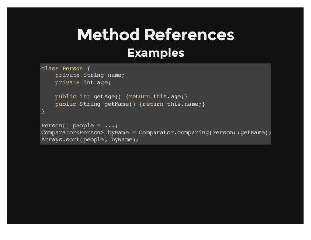
But the :: symbol can also be used for creating new Object which is called method reference :

Supplier<Apple> c1 = Apple::new;
Apple a1 = c1.get();

//== 

Supplier<Apple> c1 = () -> new Apple();
Apple a1 = c1.get();

If Apple's Constructor signature is Apple(Integer weight)，then Function should be used :

Function<Integer, Apple> c2 = Apple::new;
Apple a2 = c2.apply(110);

//== 

Function<Integer, Apple> c2 = (weight) -> new Apple(weight);
Apple a2 = c2.apply(110);

If Apple's Contructor has 2 paramters, then BiFunction should be used :

BiFunction<String, Integer, Apple> c3 = Apple::new; // point to the 2 params constructor
Apple c3 = c3.apply("green", 110); // create a new Apple object

// ==

BiFunction<String, Integer, Apple> c3 =(color, weight) -> new Apple(color, weight);
Apple c3 = c3.apply("green", 110);

So In a word, those interfaces Supplier, Function, BiFunction only create a reference to certain constructors, and the creation of new object is done by those methods get and apply. 

Well, most of the time , 2 params constructor encapsulation is enough , but what if 3,  4 .. params constructors are needed. Just define your interface like this :

public interface TriFunction<T, U, V, R>{
    R apply(T t, U u, V v);
}

And Use it similarly :

TriFunction<Integer, Integer, Integer, Color> colorFactory = Color::new;

Ok, That's all about the method reference. I will cover most of the use cases in later articles.

Java 8 -Predicate

In Java 8 , you may notice here and there some new interfaces popping out making us so unfamilar with. Well , Don't be panic. Actually, they are just some normal java syntaxs we learned before with a new name. In this article , I will tell one interface called predicate<T>.

Predicate is just a java interface with one method with return type "boolean". That's it . So , do we really need it  in java api rather than we just randomly create a interface with one method with return type "boolean". Yes, we can , we don't need it at all in java api ,but since java api helps us creating one . So we just use it.

public interface Predicate<T> {
    boolean test(T t);
}

So what is it used for ?

Well, it help us to filter some result based on the Class.  Let's see an example below.

public class MainMethod {
 public static void main(String[] args)  {

            // filter the result == 123
List<String> result123 = filter(new ArrayList<String>(), 

                             (String input) -> input.equals("123")); 

                 
 }
 
 
 public static  List<String> filter(List<String> list, Predicate<String> filter) {
  List<String> result = new ArrayList<>();
  for(String item: list)  {
      if( filter.test(item) )  {
   result.add(item);
             }
  }
       return result;
  }
}

This program filter those results with a (String == 123). So we can call filter(...) function with one paramter called Predicate,  then we specify the filter criteria when we call this function.

Alright , That's so simple to use. Well you may wonder why do we need predicate here rather than use boolean to write this function like filter (List<String> list, boolean filter) ?

Because predicate is to filter & judge a Class's field  not just a simple field :

 public static void main(String[] args)  {
  
            List<Apple> result123 = filter(new ArrayList<Apple>(), 

                     (Apple input) -> input.weight() > 100);

     List<Apple> result123 = filter(new ArrayList<Apple>(), 

                     (Apple input) -> input.color().contain("red"));
  
 }
 
 
 public static  List<String> filter(List<Apple> list, Predicate<Apple> filter) {
  List<Apple> result = new ArrayList<>();
  for(String item: list)  {
     if( filter.test(item) )  {
   result.add(item);
     }
  }
   return result;
  }

Moreover, it is more readable for you as well if you use predicate<Apple> .

Data Visulization

Data visualization is one of the important processes for data analysis. Because sometimes you may need to see whether your tuning goes to the right direction rather than wrong directions which the result looks more blur and abstract. Also, Visulization can help you demostrate your work to client and show your effort to your boss, as we human are visual animals.

Personally , I did seldom visulizations as i think they are too exaggerating and abstract which give few help to my work. But I will still show something in this article .

I will take the example from last article "cnn to train digit recognition" to visulise the convolution kernel and some output there. so the codes below can be appended after the last block following that article.

1. Kernel shape

# visualize weights
import numpy as np
W = model.layers[0].kernel.get_value(borrow=True)
W = np.squeeze(W)
print ("W shape : " , W.shape)

W shape :  (3, 3, 32)

W[:,:,0] # print the content of 1st convolution kernel

array([[ 0.04594247,  0.03799061, -0.1205595 ],
       [ 0.11602765, -0.08880974,  0.04387789],
       [-0.06434739,  0.0857822 ,  0.09397142]], dtype=float32)

2. Visualize the convolution kernel

# draw out the convolution kernel
%matplotlib inline
import matplotlib.pyplot as plt

for i in range(32):
    sub = plt.subplot(4,8,i+1) # row 4, column 8, ith image 
    plt.axis('off')
    sub.imshow(W[:,:,i], cmap=plt.cm.gray)

3. Print the shape after image is convolved by kernel

# output after convolution
import theano

convout1_f = theano.function(model.inputs,[convout1.output])
C1 = convout1_f([x_train[0]])
C1 = np.squeeze(C1)
print("C1 Shape : ", C1.shape)

C1 Shape :  (6, 6, 32)

Here you may need to install the theano by the way.

4. Visualize image after convolved by the kernel

%matplotlib inline
import matplotlib.pyplot as plt

for i in range(32):
    sub = plt.subplot(4,8,i+1)
    plt.axis('off')
    sub.imshow(C1[:,:,i], cmap=plt.cm.gray)

Oracle "View"

View = A dummy table. if a view contains only data from one table . then , the data update in the table will auto-update the data in view.

Grammar；

Create [or replace] [force] view view1 as select * from  student [ with check option] [with read only]; 

force : create a view by force , don't care whether the table is existed or not!
with check option : don't allow any update to make the data in view increase or decrease.
with read only : don't allow any update , read only.

Concatenating view :

Join multiple tables to create a view is called cancatenating view, you can do DML to columns in key-preserved table but can't update columns in non key-preserved table.

key-preserved table : the primary key in one table is regared as the primary key in view.
non key-preserved table : the primary key in the rest tables are not regarded as the primary key of view.

Create view view_student_address1 as select s.sno  sno1,s.sname, s.sno sno2, a.zz from student1 s, address a where s.sno = a.sno;  // create a concatenating view

Update view_student_address1 set sno1 = 12 where sno1 = 2; // can update, because it belongs to key-preserved table

If you want to update the data in non key-preserved table,  the only thing you can do is to use Oracle's instead of trigger, it can manipulate any view.

Hope my article can help you in your work.

Using CCN to train digit recognition

Convolution neural network is known as the most accurate model to train the digit recognition, When in college , we learned laplace transformation in convolution therem . Well I think everyone has return that knowledge to your teacher and leave nothing in your brain. That's ok . So am I. However, we don't need to implement the CNN from stratch and train the data. The keras has already done the model so that we can easily use to trigger the traing in just a few steps.

1. Import Data

import keras
import pandas as pd
from keras import backend as K
from keras.models import Sequential
from keras.layers import Dense, Dropout,Flatten
from keras.layers import Conv2D, MaxPooling2D
from sklearn.model_selection import train_test_split

# Import Data
dataset = pd.read_csv("train.csv")
target = dataset.iloc[:,0].values.ravel()
train = dataset.iloc[:,1:].values
test = pd.read_csv("test.csv").values.reshape(-1,28,28,1)

data_x = train # feartures
data_y = target # targets

x_train, x_test, y_train, y_test = train_test_split(data_x, data_y, test_size=0.2, random_state=42) # split the data
print (x_train.shape);

(33600, 784)

2.Reshape Data

Reshaping data is important as the CNN in Keras only can take data with certain shape. So we have no chices but to reshape the input data.

# 10 numbers 

num_classes = 10  

# input image dimensions
img_rows, img_cols = 28, 28

if K.image_data_format() == 'channels_first':
    x_train = x_train.reshape(x_train.shape[0],1,img_rows,img_cols)
    x_test = x_test.reshape(x_test.shape[0],1,img_rows,img_cols)
    input_shape = (1,img_rows,img_cols)  # 3 = RGB， 1 = black & white
    print (input_shape)
else:
    x_train = x_train.reshape(x_train.shape[0],img_rows,img_cols,1)
    x_test = x_test.reshape(x_test.shape[0],img_rows,img_cols,1)
    input_shape = (img_rows,img_cols,1)
    print (input_shape)


(28, 28, 1)


3. Transfer the integer into 0~1 decimal numbers






# 0~1 float

x_train = x_train.astype("float32")
x_test  = x_test.astype("float32")
x_train /= 255
x_test  /=255 

print('x_train shape:', x_train.shape)
print(x_train.shape[0], 'train samples')
print(x_test.shape[0], 'test samples')





4. Set some basic params for the CNN

y_train = keras.utils.to_categorical(y_train,num_classes) # one-hot encoder
y_test = keras.utils.to_categorical(y_test,num_classes) # one-hot encoder

model =Sequential()
model.add(Conv2D(32, kernel_size=(3,3), activation='relu',input_shape=input_shape)) #32C3
          
model.add(Conv2D(64, kernel_size=(3,3), activation='relu')) #64C3

model.add(MaxPooling2D(pool_size=(2,2))) #MP2
model.add(Dropout(0.25))

model.add(Flatten())
model.add(Dense(128,activation='relu')) # Dense must has Flatten in front ,                                 Total Chain : 6C5-MP2-16C5-MP2-120C1 (FLATTEN) -84N-10N

model.add(Dropout(0.5))
model.add(Dense(num_classes,activation='softmax'))

model.compile(loss=keras.losses.categorical_crossentropy,
              optimizer=keras.optimizers.Adadelta(),
              metrics=['accuracy'])







5. Train the model



The batch_size and epoch are needed to be tuned, here I just randomly give 2 number for demostration.

history = model.fit(x_train, y_train, batch_size=200, epochs=12, verbose=1, validation_data=(x_test, y_test))
score = model.evaluate(x_test, y_test, verbose=0)



6. Draw a graph

%matplotlib inline

import matplotlib
import matplotlib.pyplot as plt


plt.xlabel('x')
plt.ylabel('y')
plt.title('accuracy graph')

plt.plot(range(len(history.history['val_acc'])), history.history['val_acc'])

plt.show()

7.Predict

y_pred = model.predict_classes(test) ## predict, = predict

np.savetxt('CNN_6.csv', np.c_[range(1,len(test)+1),y_pred], delimiter=',', 
           header = 'ImageId,Label', comments = '', fmt='%d')

Well, Why not upload your CNN_6.csv to kaggle to see how the result goes . If the params are properly given , the result should be good enough.

A good table structure can avoid all tunings.

       is the recommendation i give for this topic.

Table structure design is the first step for people to create an application. However becuase some company / people has limited knowledge on database, when their application was put in production, It has bugs and errors here and there. And the oracle is keep releasing from  8i 9i 10G 11G 12C onwards, some bugs has been fixed , some algorithums has been improved, they are still blur on that . 

One obvious case in my work,  when in 10G , the data type char and Varchar2 have some efficiency issues which make these 2 data type different . Thus DBA in oracle 10G are more apt to char rather than varchar2, However, in 11G which is the version i am current using , this problem has been fixed by Oracle , so varchar2 has a better performance than char and also can tolerate a longer String length. And char has been put in the deprecated list in later releases. When I see the table design by our DBA , they are still using char to improve certain performance. Similar cases appear very often . 

In this article , I won't dig so much on these details ,  I will share some important points on table design and how these points can affect queries.

Index Foreign key : 

If tables linked by pri-for key, then don't remember add index on foreign key.

3 ways of Oracle partitioning : 

• range partitioning
• list partitioning
• hash partitioning

3 combined ways of partitioning:

• range-range
• list-list
• list-hash

2 types of index :

• local index , index on partitons : create index .... local;
• global index, index on tables

Why do we need to create partitions?

Because , we can narrow down the scan range when we query so as to improve the speed, Also, It's easier to clean those partitons (truncate, drop, split,add,exchange), Delete will occupy lots of rollback segments writing into undo tablespace those deleted data. so when we clean partitions, we don't need to delete the whole table , so it is very convenient. 

eg:

Alter table t truncate/drop p1; 
Alter table t split partition p_default at 3000 into (partition p3,partition p4);
Alter table t add partition p6 values less than (6000); // delete maxvalue before do it
Alter table t1 exchange partition p1 with table t2 including indexes update global indexes; // exchange data between 2 tables. 

partition table & rowid : when you do an update in partition table, the rowid will be changed as well.
Global tempprary table : auto-cleased when session is closed or transaction is commited
IOT and cluster table : when query an IOT , it won't query from your original table , add index in columns with order by and foreign key.

Primary key : this is just (an index + a constrain), we can directly change an index into a primary key.

Alter table t add  constraint ord_pk primary key(order_id,item_id) using index ord_idx;

Table compression : This will decrease the logic read but increase the CPU.

Alter table t move compress;
Execute dbms.gather_table_stats(ownname=>user,tabname=>'T');
Select table_name, blocks, cp,ression from user_tables where table_name='T';

Never use char and long .

Drop truncate add spilt exchange // this will make index invalidated
Alter table table1 drop partition p1 update global indexes; // this can avoid index invalidated
Alter index idx_par_1 rebuild partition p3; //rebuild local index

collect statistics :

Alter session set statstics_level=all;
Select * from t1,t2 where t1.id=t2.t1_id;
Select * from table(dbms_xplan.display_cursor(null,null,'allstats last'));

Replace delete table with global temporary table:

This can reduce the blow of redo log .

Create global temporary table t_global (id int, col2 int) on commit delete rows;
Insert into t_global.....
//other manipulations ....
commit;

In real situation , we wrote some script to monitor rather than wait for the problems to come out . Scripts are too long to share here, if you have any problem ,please leave a msg.

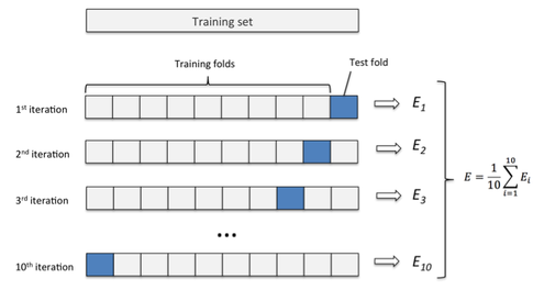
StratifiedKFold vs Normal KFold

StratifiedKFold is a kind of advanced KFold， the Normal KFold process is as below as we know.

x_data = np.array([[1,2],[2,4],[3,2],[4,4],[5,4],[6,2],[7,4],[8,4],[9,2],[10,4],[11,2],[12,4],[13,2],[14,4],[15,4]
                  ,[16,2],[17,4],[18,4],[19,2],[20,4]])
y_data = np.array([1,2,3,4,5,1,2,3,4,5,1,2,3,4,5,1,2,3,4,5])

kf = KFold(n_splits=10)

for train_index, test_index in kf.split(x_data):
    x_train = x_data[train_index]
    y_train = y_data[train_index]
    x_test = x_data[test_index]
    t_text = y_data[test_index]
    print ("train:{0}  test:{1}".format(train_index,test_index))
    
    # train model
    # test model 
    # get error rate

train:[ 2  3  4  5  6  7  8  9 10 11 12 13 14 15 16 17 18 19]  test:[0 1]
train:[ 0  1  4  5  6  7  8  9 10 11 12 13 14 15 16 17 18 19]  test:[2 3]
train:[ 0  1  2  3  6  7  8  9 10 11 12 13 14 15 16 17 18 19]  test:[4 5]
train:[ 0  1  2  3  4  5  8  9 10 11 12 13 14 15 16 17 18 19]  test:[6 7]
train:[ 0  1  2  3  4  5  6  7 10 11 12 13 14 15 16 17 18 19]  test:[8 9]
train:[ 0  1  2  3  4  5  6  7  8  9 12 13 14 15 16 17 18 19]  test:[10 11]
train:[ 0  1  2  3  4  5  6  7  8  9 10 11 14 15 16 17 18 19]  test:[12 13]
train:[ 0  1  2  3  4  5  6  7  8  9 10 11 12 13 16 17 18 19]  test:[14 15]
train:[ 0  1  2  3  4  5  6  7  8  9 10 11 12 13 14 15 18 19]  test:[16 17]
train:[ 0  1  2  3  4  5  6  7  8  9 10 11 12 13 14 15 16 17]  test:[18 19]

Well , you may notice that the test data don't give a complete categorization . only 2.

However for the stratifiedKFold, it's as below:

x_data = np.array([[1,2],[2,4],[3,2],[4,4],[5,4],[6,2],[7,4],[8,4],[9,2],[10,4],[11,2],[12,4],[13,2],[14,4],[15,4]
                  ,[16,2],[17,4],[18,4],[19,2],[20,4]])
y_data = np.array([1,2,3,4,5,1,2,3,4,5,1,2,3,4,5,1,2,3,4,5])

# in each fold , test set will contain 1,2,3,4,5 completed data, so K is set maximumly to 4 here
kf = StratifiedKFold(n_splits=4)

for train_index, test_index in kf.split(x_data,y_data):
    x_train = x_data[train_index]
    y_train = y_data[train_index]
    x_test = x_data[test_index]
    t_text = y_data[test_index]
    print ("train:{0}  test:{1}".format(train_index,test_index))
    
    # train model
    # test model 
    # get error rate

train:[ 5  6  7  8  9 10 11 12 13 14 15 16 17 18 19]  test:[0 1 2 3 4]
train:[ 0  1  2  3  4 10 11 12 13 14 15 16 17 18 19]  test:[5 6 7 8 9]
train:[ 0  1  2  3  4  5  6  7  8  9 15 16 17 18 19]  test:[10 11 12 13 14]
train:[ 0  1  2  3  4  5  6  7  8  9 10 11 12 13 14]  test:[15 16 17 18 19]

Now, It's very comprehensive. So normally we choose StratifiedKFold rather than Normal KFold.